
Have you ever found yourself in a situation where you need to filter a set of transactions based on categories which need to be calculated from that same set?
Let’s say you have a data set containing all the customer responses triggered by your Marketing activity and you need to rank Marketing campaigns performance based on the number of first touch responses they originated.
Another example more familiar to Tableau users: you have a full list of orders with line items from the Superstore data set and you need to filter customers based on the largest item’s product family they bought on their most recent order… Or how about showing on a map the revenue of customers who have been inactive for a year or more, based on the shipping address of their last order?
All those scenarios revolve around the same meta problem: the need to switch between different levels of aggregated data within the same process. In other words, the filter is computed on a subset of the transactions, and we need to run that filter without destroying any information, nor storing the same information multiple times, which could work, but would be resource intensive and frankly inelegant.
The better approach requires a database engine (sorry Excel cave folks!): by combining a series of INDB tricks and SQL functions, this can be done in a couple of easy clicks with great performance, at no additional storage cost.
Let’s use that Superstore data set for illustration, with the following scenario:
As I am preparing a promotion on Technology products, I need a list of customers who purchased over $100 worth of Technology Product Category on their last Order, to email them that promotion. In order to prepare those emails, I want to research their purchase history, with a basket analysis for instance. Therefore, I need all the order line items for that subset of customers. If I run that promotion multiple times, or if I run another similar promotion with slightly different criteria, I would really benefit from having a clean Alteryx workflow to run at will with updated data sets.
I will run Window Functions on Snowflake because that Cloud DB is so easy to provision, and I recently published a guide to get you started as well, but you could use the same Window Functions on most modern databases. Here are the references for some of the DBs I have been using:
- MS SQL Server and Azure SQL: Official documentation and a better resource
- AWS Redshift: Official documentation
- PostGres: Official Documentation and a good explainer of the concepts
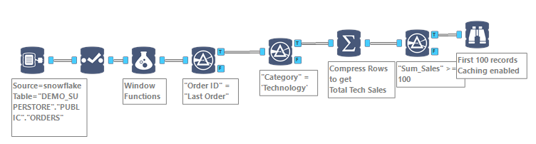
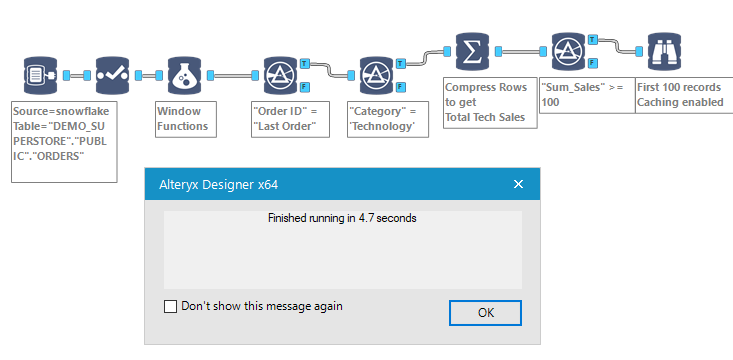
Upon loading the Superstore Sales in Snowflake, we are getting 9,994 rows of Order Line items, from 793 distinct Customer IDs. We will first attempt to isolate those customers, whose last Order comprised at least $100 of Technology items. As you will see below, the workflow is quite streamlined:
 The Formula object is where the magic happens, calculating those aggregate indicators we need:
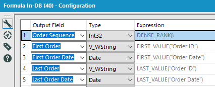 Here is the code I used for Snowflake INDB:
- Order Sequence:
DENSE_RANK()
OVER (PARTITION BY “Customer ID”
ORDER by “Customer ID”,”Order ID”,”Order Date”) - First Order:
FIRST_VALUE(“Order ID”)
OVER (PARTITION BY “Customer ID”
ORDER by “Customer ID”,”Order ID”,”Order Date”) - First Order Date:
FIRST_VALUE(“Order Date”)
OVER (PARTITION BY “Customer ID”
ORDER by “Customer ID”,”Order ID”,”Order Date”) - Last Order:
LAST_VALUE(“Order ID”)
OVER (PARTITION BY “Customer ID”
ORDER by “Customer ID”,”Order ID”,”Order Date”) - Last Order Date:
LAST_VALUE(“Order Date”)
OVER (PARTITION BY “Customer ID”
ORDER by “Customer ID”,”Order ID”,”Order Date”)
Note that some SQL versions, I’m looking at you Microsoft, require for the LAST_VALUE function to operate correctly, to specify a ROW or RANGE clause, as the windows default clause associated with ORDER BY is too restricted. If you get into that issue, finding weird results for your Most Recent values, insert ROWS BETWEEN CURRENT ROW AND UNBOUNDED FOLLOWING before you close the bracket, like that:
LAST_VALUE(“Order ID”)
OVER (PARTITION BY “Customer ID”
ORDER by “Customer ID”,”Order ID”,”Order Date”
ROWS BETWEEN CURRENT ROW AND UNBOUNDED FOLLOWING)
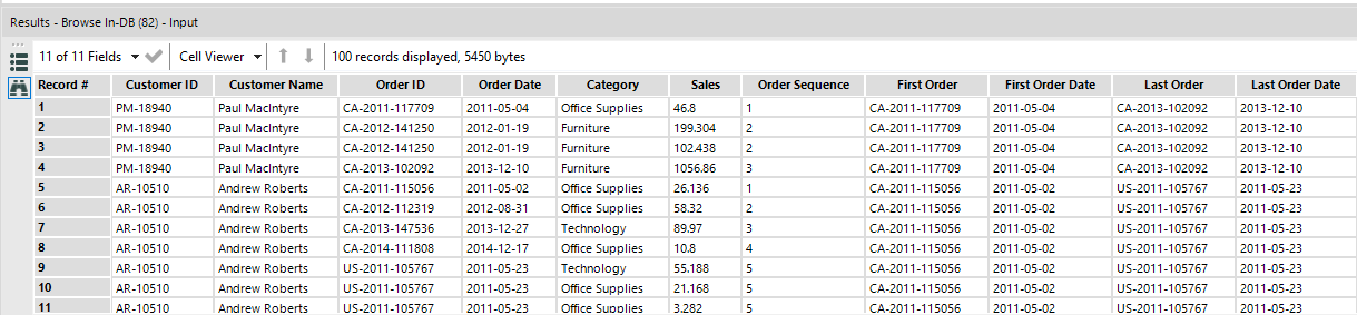
Upon correct code, I obtain those 5 new columns on my data set:
 Then I can filter Order line items to only the last Order with a simple Filter tool to get down to 1,646 line items for those 793 customers:
“Order ID” = “Last Order”
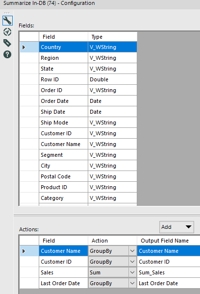
All I have to do next is to filter on Technology Category, getting down to 257 customers and compress rows using the Summarize tool:
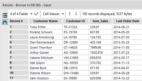
 Now I can filter those customers with the sum of Technology sales on their last order > $100, to get down to the final list of 165 customers, looking like this:
The workflow, on the smallest available Snowflake instance, runs really fast, even if you have a much larger Order data set:
Now, I can append any Customer level or Order level attribute to that summary. More important, I can now use that temp table to filter the whole data set, to pull the full order history of those 165 customers per the scenario above, using their Customer ID:
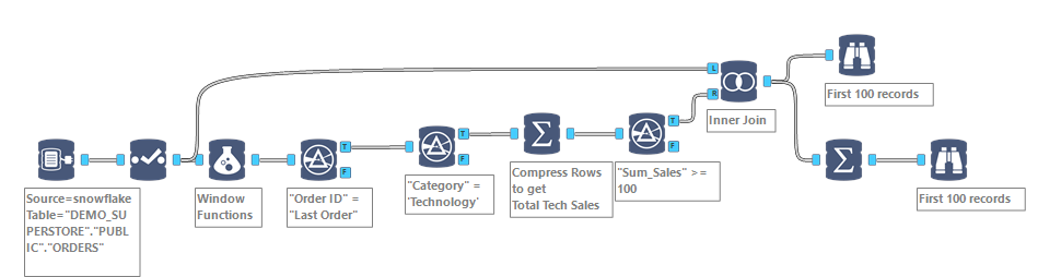 Using that simple additional Join In-DB tool on Customer ID, I retrieve for those 165 relevant customers 2,165 Order Line items, ready for analysis.
Those techniques open so many possibilities to handle aggregation levels, that I highly recommend you reproduce those steps on your own, to get familiar with those precious Window Functions.
Pingback: Customer Cohorts and Product Sequence with orders data | Insights Through Data
Pingback: How to Concatenate Strings in Snowflake with Alteryx INDB | Insights Through Data