
If you are still manipulating data in Excel, why should you care about In-DB and Redshift? Whether you are accessing your Redshift data through Alteryx or through Tableau, knowing how to prepare your data within Redshift, with In-DB tool in Alteryx or with a prep query in the Tableau connector to Redshift, will give you access to another level of performance and flexibility. Even though it might sound to you like science fiction, it is not… These are just Redshift functions you can run through ODBC…
Having a Database to read from and write to, is really nice when using Alteryx, even though you can make do without, with local .YXDB files. The key benefit of a dedicated database is the ability to use In-DB tools. Working In-DB saves the time it takes to import and export data to and from the Alteryx engine memory, and leverages the power of the DB engine. Shifting an analyst’s data Field of Play to a Massively Parallel Processing (MPP) Database such as Redshift, brings additional performance improvements. I would deem those gains massive: I have seen 6 minutes Alteryx workflows run in 15 seconds In-DB. Note that besides Redshift, the following databases are supported In-DB by Alteryx:
- Cloudera Impala
- Databricks
- Hive
- Microsoft Azure SQL Data Warehouse
- Microsoft SQL Server
- Oracle
- Spark
- Teradata
For all the wonders of the Alteryx data engine, which never seems to choke on anything sent its way for processing, it cannot really compete with the parallel processing of Redshift, when used In-DB. From an analyst perspective, there are some trade-offs for the additional performance, scale and efficiency. Main one is the steep initial learning curve, since it requires the adoption of a wholly different set of tools. Furthermore, you will quickly find that those tools have limitations, inherent to the underlying SQL operations generated through ODBC. The 10 tricks of this post will hopefully alleviate some of those difficulties. If you’re still not too sure about your SQL operations. Check out red9 for any further support.
In order not to lose beginners, I attempted to rank these 10 tips by gradual order of complexity, whether conceptually or implementation wise. That grading will hopefully compel readers to progress through the adoption of In-DB processing. But before I start, some preliminary observations on the inner workings of In-DB.
If you are used to process your data in Alteryx in memory, you have adopted a very sequential way of thinking: Take data from this source, apply this tool, then that one and so forth, until the expected results. In-DB looks deceptively similar: insert a data source, then add tools to get to the expected results. However, notice that when the In-DB workflow runs, you don’t see the progress of rows processed. Contrary to a regular workflow which takes place mostly sequentially in Alteryx memory, a workflow featuring several In-DB tools between the Stream In and the Stream Out tools, sends a single massive SQL query to Redshift through ODBC. One downside is that, when you create a new column with a formula, it may happen that another tool further down the workflow will not know that column yet. Try to keep only one column per formula tool. First trick will help exposing further the difference in approach.
1. Use aggregates to track progress through workflow
One of the downsides of simultaneous processing of In-DB is that you can’t see progress of data along the workflow during its run. It makes it hard to check the granularity of the manipulated data at various stages. The obvious way to control that, is to add Browse In-DB tools along the way. And do yourself a favor, disable the cache button which is enabled by default:
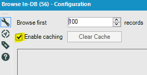
The minor performance gains while you develop are not worth your confusion when the expected changes you make to the workflow, don’t materialize in Browse because of caching, and the ensuing face palm…
Also, note that the Browse tool In-DB is very taxing to the Alteryx engine, as it requires to import the data into Alteryx memory for browsing. A much better approach is to use the Summarize In-DB tool along the way, with a Count of the table keys, and a Distinct Count for safety. That tool can then be copied/pasted and positioned at strategic inflections of the process, during the development/ test phase. This won’t tax your performance so much, since DB engines are optimized for aggregates.
2. Time filters
The Filter tool is essential In-DB, but it tends to be tricky compared to the comfort of the regular in memory Filter tool, especially when dealing with dates. Here is the syntax for a basic filter to take all records since Nov 20, 2016:
“CreatedDate” >= ‘2016-11-20’
A more advanced filter to select the last 5 days including today:
“CreatedDate” >= dateadd(day,-5,’today’)
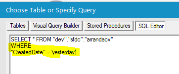
Redshift will also accept this syntax:
“CreatedDate” = ‘yesterday’
There is a wealth of additional time functions to calculate fancy intervals.
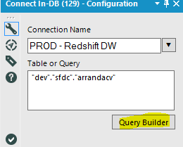
Note that you are better off inserting your filter code into the Redshift connector if you can, rather than in a separate Filter tool. Under the hood, Alteryx generates one massive Redshift SQL queries, comprising of a series of CTEs (Common Table Expressions), one embedded for each tool. Instead of doing a Select * on your source table, and then another Select on the resulting table, you are better off performing the Select early, and work with less rows down the workflow. In the connector, click on Query Builder:
 Then SQL editor, and insert your WHERE clause:
3. Conditions
In your workflows, chances are you are using conditional statements in a formula quite often, to create categories or bins for instance. In regular in memory Alteryx, you are offered a choice:
a. Boolean condition using IIF(bool, x, y) which is equivalent to the IF() function in Excel. Example:
IIF([Age]>50,’Old’,’Young’)
Nice and easy but quite limited…
b. A more flexible option is to use IF c THEN t ELSEIF c2 THEN t2 ELSE f ENDIF which can accommodate more than one alternative, using ELSEIF. Example:
IF [Age]>70 THEN ‘Retired’
ELSEIF [Age]>50 THEN ‘Senior’
ELSEIF [Age]>0 THEN ‘Young’
ELSE ‘No Age available’
ENDIF
Tableau is matching Alteryx, and offers a third option with CASE:
a. Boolean: IIF(test, then, else, [unknown])
b. Flexible: IF test1 THEN value1 ELSEIF test2 THEN value2 ELSE else END
c. Ultimate with the CASE statement: CASE expression WHEN value1 THEN return1 WHEN value2 THEN return2…ELSE default return END to accommodate many alternatives, while keeping the code easy to read and maintain:
CASE [Age]
WHEN “age”>70 THEN “Retired”
WHEN “age”>50 THEN “Senior”
WHEN “age”>0 THEN “Young”
ELSE “No Age available”
END
Redshift, and therefore Alteryx In-DB offers only one option, thankfully the most powerful, the Case statement, using this syntax, very similar to Tableau’s:
Case “age”
When “age”>70 THEN ‘Retired’
When “age”>50 THEN ‘Senior’
When “age”>0 THEN ‘Young’
ELSE ‘No Age available’
END
4. Concatenate
To create a compound key or attribute is fairly easy with a regular formula tool:
[First Name]+’ ‘+[Last Name]
with the In-DB Formula tool, the Concatenate function is required, using this syntax:
“First Name”||’ ‘||”Last Name”
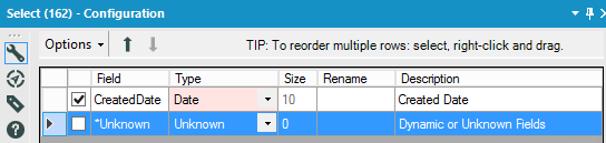
5. Change Data Type
To change the Data Type in Alteryx is fairly easy with the Select tool, from DateTime to Date for instance, using the Type Drop Down:
 With In-DB, it takes a Formula and the CAST function:
“createddate” :: date
6. Fill in the blanks
A regular Alteryx formula would use a simple Boolean test:
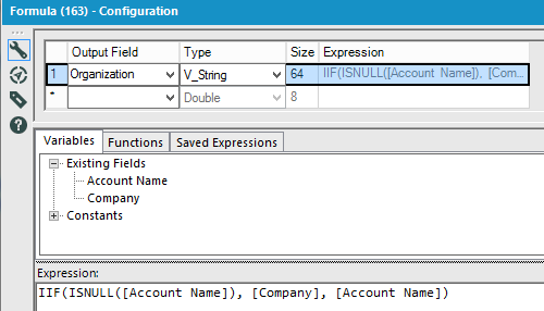
Redshift requires the use of the NVL function, for the Organization field in that example:
NVL(“Account Name”,”Company”)
That function replaces NULLs with the first non Null value found in the indicated columns on that same line. It is a bit more powerful, as several columns can be added in the test at once, which would take a IF function with several ELSEIFs, using a regular formula.
7. Sort a table
Sorting data in Redshift In-DB deserves its own trick number? Well, check the In-DB tool set, there is no Sort tool. Fortunately, you can hack your way through, by using the In-DB Sample tool that way:
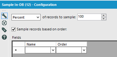
It’s a bit convoluted, but it works…
8. Filter on a string of text
Regular in memory Alteryx has a variety of functions to filter or just plainly search a string, such as FindString(String, Target) or Contains(String, Target). For In-DB Redshift, there is REGEXP_INSTR, but the POSITION function is easier to use than REGEX. Let’s say I need to find all orders featuring a blue item, I could filter the line item description in the order table using this syntax:
POSITION(‘blue’ IN “Line Item Description” )=0
0 implies not found, so I would plug the workflow to the F (for False) exit of the Alteryx In-DB Filter tool. This is pretty much equivalent to a CONTAINS function in Tableau.
9. Excluding Joints
We are entering more complex tricks here, and this one builds on a previous post where I was explaining how to translate SQL joins into Alteryx regular tools language, mostly the Join tool. As you saw in that previous post, Alteryx makes it easy to accommodate the 7 types of Joints you can be expected to use:
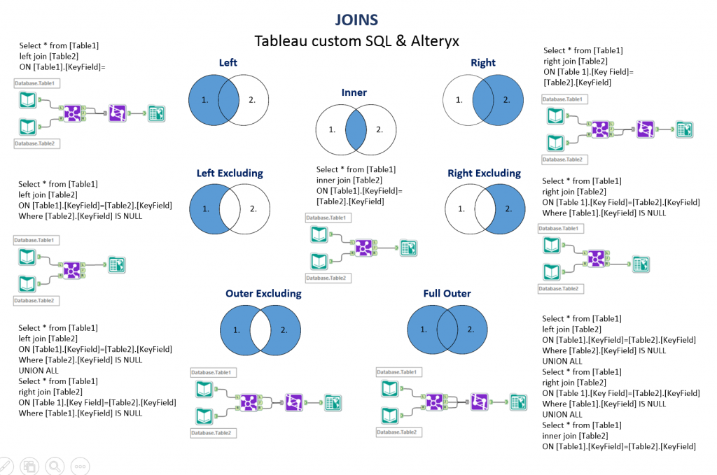
Information Labs’ excellent cheat sheet
Yet, when taking a look at the In-DB Join tool, something is missing:
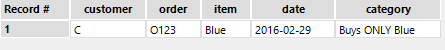
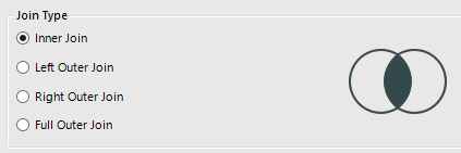 Where are the 3 Excluding Joints: Left, Right and Outer? Do I really need them? Let me illustrate with a business scenario. Let’s say I have in my Redshift DB a bunch of customer orders, that look like this:
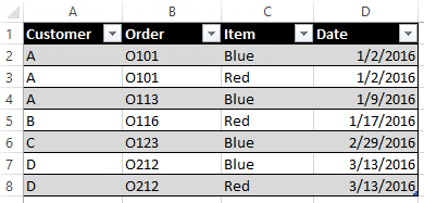 I need to count how many Customers have bought ONLY the blue item. If I filter transactions to Blue, and aggregate Customers, I will have 3 Customers in my count: A, C and D: wrong answer! Only C qualifies…
I will need to get fancier, by using an Excluding Joint, to exclude from the Customers who bought Blue, those who ALSO bought Red, to be down to those who bought strictly Red:
Will I have to inject some SQL in my workflow and break the existing complex query Alteryx is sending through ODBC? Sounds like a mess… There is actually a fairly simple solution out of this predicament with In-DB, once you know it, a 3 tools combo: Left Outer Join + Filter + Select
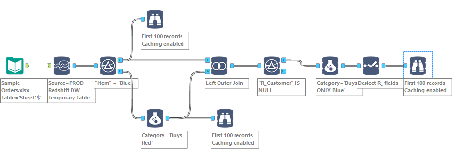 Any In-DB Joins produce R_ (for Right origin) fields, which can be used as a filter to reject the overlapping of the Join in a filter. Then all there is left to do is take those R_ fields out with a Select… Instead of this wrong result post Blue Filter:
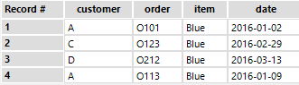 I am getting this:
10. Last but not least: Replace the Unique Tool and take control of the granularity
I mentioned it before, I LOVE the Unique tool, which proudly sits in my Alteryx favorites:

I’ll be the first to admit it, it is not very SQL observant, but it is such a convenient tool, boosting productivity greatly, when used in combo with the Sort tool. To begin with, you will notice that among In-DB tools, there is no Unique tool, and no Sort tool… We saw above a hack to sort the table, not very elegant, but convenient… Not good enough for many scenarii though… Let’s use the same sample of Orders used above, but this time, the scenario is: how to get a list of only the first orders Customers filed in 2016, with all the attributes of those orders? In that sample, I would need to exclude Order O113, since Customer A already purchased O101 in 2016:
This rules out the simple approach of using Summarize with a Min/Max on Order date, because I would discard which items were found in the order. All the relevant line items and their attributes are needed… If only I could sort my orders by date, and simply use Unique on Customer + Order… To prevail, we will need to dive deeper into the depths of Redshift, and leverage Redshift Window functions…
 The first step is to identify the time rank of orders and stamp every line items (=rows) under the order with the rank. Here is the formula for my OrderSequence column, leveraging the window Dense_Rank function:
dense_rank() over (partition by “customer” order by “customer”,”order”,”date” )
and here is the result:
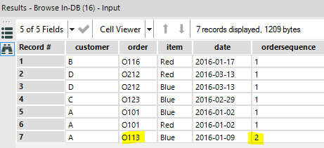 All I have to do from there is to filter out the orders ranked higher than 1, to take out O113. Note that had I used a simple window Rank function, I would have obtained the intended results as well, but line items in O113 would have been ranked 3, and there would be no 2, since the two line items from O101 tie at rank 1.
Note that you can use the same technique to replace the Record ID tool, not available In-DB either: This time, you can use a Sum(1) function before the Over, and partition by the maximum level of granularity of the table. For instance, use Partition Line Item # for a table of Orders.
Those Window functions are a bit tough to operate initially, without practice. Here are some explanations I found helpful. Those functions are worth studying for anyone working with In-DB, just like the Tile tool for in memory Alteryx, they are a powerful tool set to leverage the power of Redshift or PostgreSQL In-DB…
Hi Frederic,
This is another excellent article and I’ll certainly be using this sometime in the future. When the Tableau Redshift connector was first released back in Oct 2013, I did some work on the platform and wrote an article that I thought nobody would ever read. Much to my surprise, it got read a lot! I think the same is going to happen to this one. This is really excellent work and thanks so much for writing it!
https://3danim8.wordpress.com/2013/10/30/insights-on-using-tableau-coupled-with-amazon-redshift/