Wean Off VLOOKUP with the Index-Match Combo

Whether you need to perform a quick & dirty join of two tables in Excel to fetch an attribute, or to build more robust (!) data blending for your data preparation, you might still be limiting yourself to just the ubiquitous VLOOKUP() Excel function.

I don’t blame you, VLOOKUP() is convenient, fairly easy to use as it has been around and is well documented, not too treacherous if you sort well and properly use the final Range_lookup Argument…

Nevertheless, there are better options out there!

<Update Jan 2020: Actually there is a brand new feature in Excel 2019 that rebuilds the concept and does away with many issues. It is a new function called XLOOKUP! More details here)

The best, imho, is Alteryx’s great Find Replace tool, full of options:

But should you need to remain within the limits of a plain version of Excel, you can improve upon VLOOKUP by using the great Index-Match combo which will beat VLOOKUP() with:

1. Improved performance, no more recalculating wait
2. Ability to select any column on the reference table, not just the first one to the left
3. Improved reliability as you select resulting column with an address or a name and therefore a formula, not just through a limited count to the right of the first column, very static and limiting

Because it is a combo, it is not as well documented as a single function like VLOOKUP() can be, but there are still plenty of good resource. In a nutshell, here is the syntax of the combo:
=INDEX(Target Result Column to Insert, MATCH(Look up Value Source,Look up Column,0))

Here is a use case illustration with a step by step  using a Superstore sample dataset :

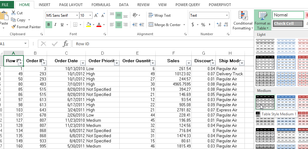
1. Format Orders and Users tab into tables to ensure integrity and ease of manipulation with Home/Format as Table:
   
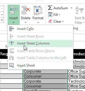
2. Insert Column to the right of column N Region and name it Manager:
   
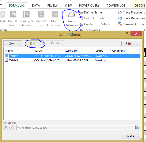
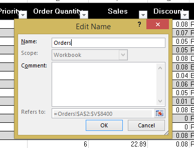
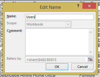
3. Go to Formulas/Name Manager and edit the two tables you created to rename them to Orders and Users:
   
4. Input in Cell O2 the following formula: =INDEX(Users[Manager],MATCH([@Region],Users[Region],0))

The Manager column should now be populated automatically by the table with the relevant Manager name read from the User tab. Note that you can insert columns left or right in either tables without breaking anything.

Here is the resulting Superstore Sales file.

<Update from September 2016>
Should you want to take the next step and enhance your Index/Match to use more than one search criteria at once, Spreadsheeto has a good tutorial to turn the formula into an Array formula, which will accommodate additional criteria:
http://spreadsheeto.com/index-match/