
When trying to get a better grip on the performance of a large number of customers (or accounts, or pupils for the matter), and progression over time of their count, their revenue or their conversion from one status to another, it really helps to organize them in cohorts, to compare them fairly. Namely, you would want to compare the 2017 revenue generated by customers who have been transecting since 2014, with the revenue of those who transact since 2016, as they are at different stage in their customer journey, hopefully. For illustration, the Tableau SuperStore data set has 793 customers and 5,009 orders over 4 years:
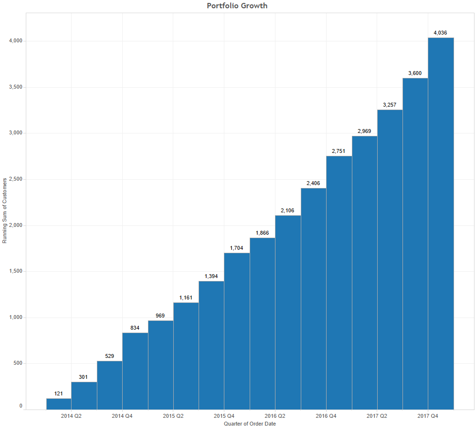
From that perspective, the growth of the number of customers looks steady and healthy, but is it really? Are we acquiring customers in 2017 as we did in 2015? Critical details, such as the number of orders per customers are buried within that mass of data.
A better angle would be to depict the progression of those customers by cohorts, taking for reference the date of their first order to group them, and plot how are they growing in subsequent years.
That very good post explains further how to handle the necessary computations:
http://tomtunguz.com/cohort-analysis-with-r/
Tomasz explains how difficult it is to plot cohorts, and for the visually inclined like me, the post is pretty hard to grasp. In a follow up post, he illustrates the resulting chart, which is likely to be featured in a slide deck:
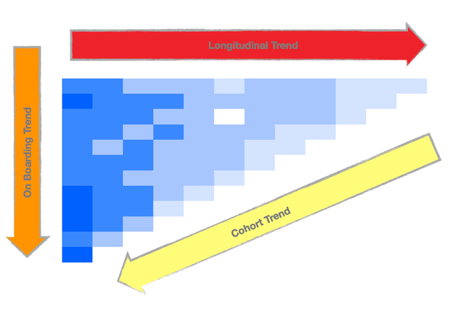
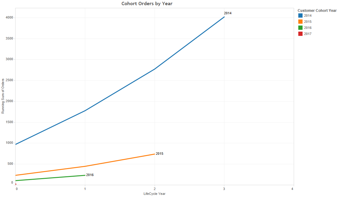
Nevertheless, I prefer an even more visual approach, which looks like this:
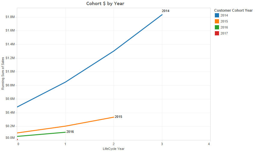 I can now compare the customers after one year of activity, that is on Year 1 of their life cycle. I can see right away that the 2014 accounts are growing must faster and stronger than the 2015 do, and 2016 perform even worse. This clearly contradicts the rosy picture of the overall portfolio growth discussed above with the first chart. If the data was real, there would be a clear cause for concern here.
I can then easily take the next step and compare them in sheer # of accounts instead of their revenue:
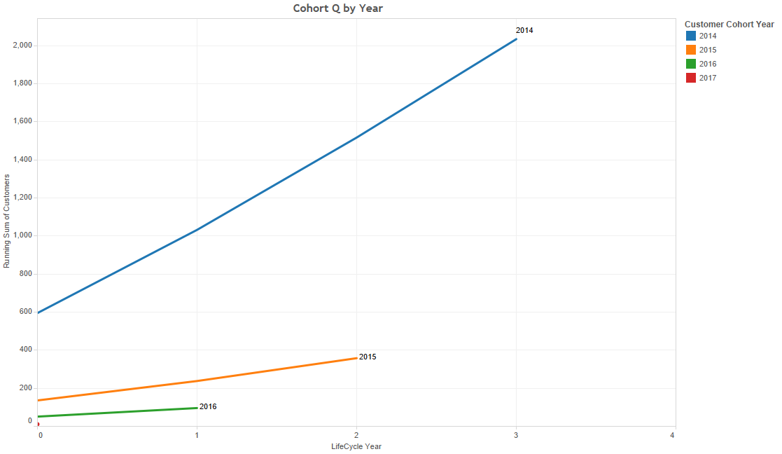
and then check whether it could be due to the volume of orders they file:
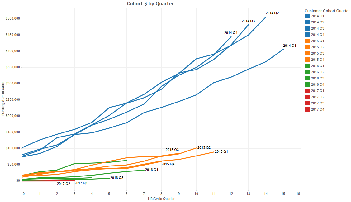
and I can easily drill down further to Quarter views, in case there is seasonality involved:
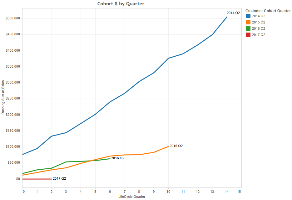
 You can then easily isolate a specific quarter with a filter:
Really, the possibilities are endless, the analysis can be performed in a matter of minutes, and it only requires a couple of formulae in Tableau. Let’s get it done!
- Step: Create the reference time stamp called Customer Since, which is the date of the first order for each customer: {FIXED [Customer Name]:MIN([Order Date])}
- Step: Create Customer Cohort Year to be used in Labels in Color Marks: DATENAME(‘year’,[Customer Since])
- Step: Create LifeCycle Year to be used in columns: datediff(‘year’,[Customer Since],[Order Date])
That’s all there is to it…
Note that if the underlying data gets updated, with new orders for instance, the graphs will include those updates, since everything is calculated on the fly while you open Tableau!
See an example workbook here.